


Basic Excel Formulas For Your Workflow
Formulas and functions are the building blocks of working with numeric data in Excel. This article introduces you to formulas and functions.
Since you’re now able to insert your preferred formulas and function correctly, let’s check some fundamental Excel functions to get you started.
1. SUM
The SUM function is the first must-know formula in Excel. It usually aggregates values from a selection of columns or rows from your selected range.
=SUM(number1, [number2], …)
Example:
=SUM(B2:G2) – A simple selection that sums the values of a row.
=SUM(A2:A8) – A simple selection that sums the values of a column.
=SUM(A2:A7, A9, A12:A15) – A sophisticated collection that sums values from range A2 to A7, skips A8, adds A9, jumps A10 and A11, then finally adds from A12 to A15.
=SUM(A2:A8)/20 – Shows you can also turn your function into a formula.

2. AVERAGE
The AVERAGE function should remind you of simple averages of data such as the average number of shareholders in a given shareholding pool.
=AVERAGE(number1, [number2], …)
Example:
=AVERAGE(B2:B11) – Shows a simple average, also similar to (SUM(B2: B11)/10)

3. COUNT
The COUNT function counts all cells in a given range that contain only numeric values.
=COUNT(value1, [value2], …)
Example:
COUNT(A:A) – Counts all values that are numerical in A column. However, you must adjust the range inside the formula to count rows.
COUNT(A1:C1) – Now it can count rows.

4. COUNTA
Like the COUNT function, COUNTA counts all cells in a given rage. However, it counts all cells regardless of type. That is, unlike COUNT that only counts numerics, it also counts dates, times, strings, logical values, errors, empty string, or text.
=COUNTA(value1, [value2], …)
Example:
COUNTA(C2:C13) – Counts rows 2 to 13 in column C regardless of type. However, like COUNT, you can’t use the same formula to count rows. You must make an adjustment to the selection inside the brackets – for example, COUNTA(C2:H2) will count columns C to H

5. IF
The IF function is often used when you want to sort your data according to a given logic. The best part of the IF formula is that you can embed formulas and function in it.
=IF(logical_test, [value_if_true], [value_if_false])
Example:
=IF(C2<D3, ‘TRUE,’ ‘FALSE’) – Checks if the value at C3 is less than the value at D3. If the logic is true, let the cell value be TRUE, else, FALSE
=IF(SUM(C1:C10) > SUM(D1:D10), SUM(C1:C10), SUM(D1:D10)) – An example of a complex IF logic. First, it sums C1 to C10 and D1 to D10, then it compares the sum. If the sum of C1 to C10 is greater than the sum of D1 to D10, then it makes the value of a cell equal to the sum of C1 to C10. Otherwise, it makes it the SUM of C1 to C10.

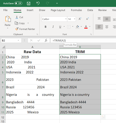
6. TRIM
The TRIM function makes sure your functions do not return errors due to unruly spaces. It ensures that all empty spaces are eliminated. Unlike other functions that can operate on a range of cells, TRIM only operates on a single cell. Therefore, it comes with the downside of adding duplicated data in your spreadsheet.
=TRIM(text)
Example:
TRIM(A2) – Removes empty spaces in the value in cell A2.
7. MAX & MIN
The MAX and MIN functions help in finding the maximum number and the minimum number in a range of values.
=MIN(number1, [number2], …)
Example:
=MIN(B2:C11) – Finds the minimum number between column B from B2 and column C from C2 to row 11 in both column B and C.
=MAX(number1, [number2], …)
Example:
=MAX(B2:C11) – Similarly, it finds the maximum number between column B from B2 and column C from C2 to row 11 in both column B and C.


* To Read other functions and formulas of ms excel visit the post:
PC Package(functions and formulas in excel)
Formulas and functions are the building blocks of working with numeric data in Excel. This article introduces you to formulas and functions.
Since you’re now able to insert your preferred formulas and function correctly, let’s check some fundamental Excel functions to get you started.
1. SUM
The SUM function is the first must-know formula in Excel. It usually aggregates values from a selection of columns or rows from your selected range.
=SUM(number1, [number2], …)
Example:
=SUM(B2:G2) – A simple selection that sums the values of a row.
=SUM(A2:A8) – A simple selection that sums the values of a column.
=SUM(A2:A7, A9, A12:A15) – A sophisticated collection that sums values from range A2 to A7, skips A8, adds A9, jumps A10 and A11, then finally adds from A12 to A15.
=SUM(A2:A8)/20 – Shows you can also turn your function into a formula.

2. AVERAGE
The AVERAGE function should remind you of simple averages of data such as the average number of shareholders in a given shareholding pool.
=AVERAGE(number1, [number2], …)
Example:
=AVERAGE(B2:B11) – Shows a simple average, also similar to (SUM(B2: B11)/10)

3. COUNT
The COUNT function counts all cells in a given range that contain only numeric values.
=COUNT(value1, [value2], …)
Example:
COUNT(A:A) – Counts all values that are numerical in A column. However, you must adjust the range inside the formula to count rows.
COUNT(A1:C1) – Now it can count rows.

4. COUNTA
Like the COUNT function, COUNTA counts all cells in a given rage. However, it counts all cells regardless of type. That is, unlike COUNT that only counts numerics, it also counts dates, times, strings, logical values, errors, empty string, or text.
=COUNTA(value1, [value2], …)
Example:
COUNTA(C2:C13) – Counts rows 2 to 13 in column C regardless of type. However, like COUNT, you can’t use the same formula to count rows. You must make an adjustment to the selection inside the brackets – for example, COUNTA(C2:H2) will count columns C to H

5. IF
The IF function is often used when you want to sort your data according to a given logic. The best part of the IF formula is that you can embed formulas and function in it.
=IF(logical_test, [value_if_true], [value_if_false])
Example:
=IF(C2<D3, ‘TRUE,’ ‘FALSE’) – Checks if the value at C3 is less than the value at D3. If the logic is true, let the cell value be TRUE, else, FALSE
=IF(SUM(C1:C10) > SUM(D1:D10), SUM(C1:C10), SUM(D1:D10)) – An example of a complex IF logic. First, it sums C1 to C10 and D1 to D10, then it compares the sum. If the sum of C1 to C10 is greater than the sum of D1 to D10, then it makes the value of a cell equal to the sum of C1 to C10. Otherwise, it makes it the SUM of C1 to C10.

6. TRIM
The TRIM function makes sure your functions do not return errors due to unruly spaces. It ensures that all empty spaces are eliminated. Unlike other functions that can operate on a range of cells, TRIM only operates on a single cell. Therefore, it comes with the downside of adding duplicated data in your spreadsheet.
=TRIM(text)
Example:
TRIM(A2) – Removes empty spaces in the value in cell A2.

7. MAX & MIN
The MAX and MIN functions help in finding the maximum number and the minimum number in a range of values.
=MIN(number1, [number2], …)
Example:
=MIN(B2:C11) – Finds the minimum number between column B from B2 and column C from C2 to row 11 in both column B and C.
=MAX(number1, [number2], …)
Example:
=MAX(B2:C11) – Similarly, it finds the maximum number between column B from B2 and column C from C2 to row 11 in both column B and C.


PC Package(functions and formulas in excel)


